In February 2024, former Syracuse head coach Jim Boeheim called out Joe Lunardi — ESPN’s lead “bracketologist,” the man who coined that term and is today the public lightning rod for all debates about NCAA Tournament selection process — for including just three ACC teams in his latest forecast for the tournament field.1 “To say there’s three teams in the tournament I don’t know what metrics you’re using. You’re using the blind man metrics is what you’re using.”
Pittsburgh head coach Jeff Capel echoed Boeheim’s complaint three days later: “I’m not a bracketology expert. I’m not a numbers expert. I know what my eyes see. It’s frustrating that a lot of people sit behind a computer and look at numbers and that’s the metrics they come up with.”2 Capel’s Panthers snuck into the 2023 tournament in the First Four as an 11-seed. They defeated Mississippi State, an SEC team ranked higher at the time in every predictive rating system, then blew out Iowa State, a Big 12 team also ranked higher at the time by every predictive rating system, before bowing out to 3-seed Xavier in the Round of 32.
The ACC’s gripes with the selection committee’s metrics have perhaps the strongest basis in NCAA Tournament results of any major conference. Per BartTorvik, the conference leads the NCAA with almost 13 more wins than expected via predictive metrics entering the tournament between 2010 and last season (2023). That number will almost assuredly rise following the conclusion of a 2024 tournament which saw the conference send three teams to the Elite Eight and an 11-seed to the Final Four. Over that same time period, the Big 12 and Mountain West — two frequent punching bags for predictive-metric critiques — have each underperformed their expectations by at least 10 wins.3
However, they are by no means the only complaints. Sometimes, the ACC isn’t the underdog hero against the elite conferences but instead a big bad Power 6 conference keeping deserving mid-majors out of the field. Just this year, Virginia received an at-large bid over an Illinois State team ranked higher by every predictive metric. The ’Hoos went scoreless for 52 minutes of real-life time and suffered a 25-point defeat to Colorado State in the First Four while Illinois State advanced to the NIT Final Four.
All this is to say that cherry-picking specific examples of teams overperforming or underperforming their metrics entering the tournament isn’t a very productive way to analyze predictive rating systems. For every 10-seed Syracuse or 11-seed NC State, there’s a 2018 Virginia to balance things out. For every 2023 FAU to assert mid-major superiority, there’s, uh, a 2024 FAU. The NCAA Tournament is random. That’s why the winner of a contest to algorithmically forecast 2022 March Madness results finished in first place without actually using any of that season’s data.4 That’s why the winner of your bracket pool will inevitably have picked their Final Four based on their favorite mascots.
What does this post do, then?
I hope to take a more systemic approach to evaluating predictive college basketball metrics in search of answering two major questions raised about these systems:
-
How big are the error bars on their team-strength estimates?
-
How does the structure of college basketball scheduling, specifically the division of teams into conferences, affect these estimates?
For this study, I’ll be “picking on” KenPom for two key reasons. First, the site is the most famous college basketball analytics page in the game right now, and probably the one most readers are familiar with. Second (and more importantly), KenPom makes its model diagnostics easily accessible, which makes it easier to construct synthetic data models to emulate KenPom.
How are we going to answer those questions?
To determine how large the margin of error is on team-strength estimates by predictive ranking systems, we’ll generate an imaginary set of 362 college basketball teams with known offensive and defensive efficiencies. Then, we’ll have each of those teams play a “typical” college basketball schedule of about 30 games. We’ll run those games through a simplified version of the adjusted-efficiency-margin system to estimate the team strengths based on our made-up season’s results. Finally, we’ll compare the estimated ratings to the known underlying ratings of each team.
To analyze the impact of the conference structure on college basketball predictive metrics, we’ll actually run this experiment four different times:
-
Each team plays 30 other teams chosen at random.
-
Each team plays 10 teams chosen at random (“non-con”) and then approximately 20 games against a “random” conference. These random conferences are assigned by taking the list of actual conference affiliations for the 2023 season and randomly assigning each conference to a team.5
-
Each team plays 10 teams chosen at random (“non-con”) and then approximately 20 games against a “true” assigned conference. The problem with Experiment 2 is that in the real world conferences aren’t assigned at random: it’s a fair bet that every year every team in the Big 12 will be better than every team in the NEC. To better reflect reality, we take the list of synthetic teams and rank them 1 to 362 by net rating. Then, we use the conferences of each team 1-362 in the final 2023 KenPom ratings to assign each synthetic team its “true” conference. For example, UConn is in the Big East and finished 1st in the 2023 KenPom ratings. So, the highest-rated team in our synthetic data is assigned to the Big East. This more accurately resembles the true structure of college basketball’s conferences.6
-
Repeat of Experiment 3, but with zero non-con games and approximately 30 conference games per team. This gives us a better look at exactly what scheduling “bubbles” does to predictive metrics by taking the example to the extreme.
In both cases, we’ll analyze how the estimated team ratings using an efficiency-ratings system compare to the true underlying team ratings in the data-generating process.
With that out of the way, let’s get into the experiment.7
Generating Synthetic Data
Before we can simulate any games, we need to invent some teams. These teams should resemble the “true” distribution of college basketball team strengths, so we’re going to literally base them on the KenPom ratings after the 2023 NCAA Tournament. As it turns out, offensive and defensive efficiencies are approximately Normally distributed — the graphs below show the distributions of offensive and defensive ratings in blue, with a Normal distribution overlaid with a mean and variance equal to the sample mean and sample variance of offensive and defensive ratings, respectively. What matters here is that these distributions match up closely enough to the observed data to generate reasonable synthetic data from a multivariate Normal distribution.
KenPom 2023 Histograms
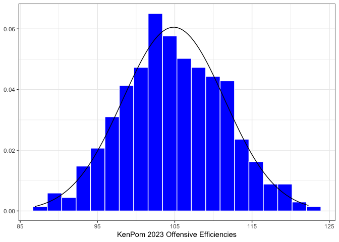
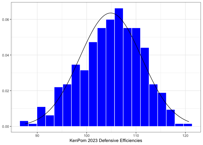
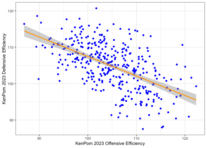
There is one caveat before we go just randomly sampling values: offensive and defensive ratings are not uncorrelated. Teams with good offenses also tend to have good defenses — something that everyone knows about basketball, and also something we can confirm at a glance from simply plotting offensive and defensive ratings against one another.
Offensive and Defensive Ratings Aren’t Independent
Generating Synthetic Data
To account for this correlation, we need to also specify the covariance
matrix of the multivariate Normal distribution based on sample variance
and covariance. Thankfully, R very handily makes it easy to sample from
multivariate Normal distributions with given means and
variance-covariance matrices using the MASS package’s mvrnorm
function.
First, we estimate the means and the variance-covariance matrix from the data:
O.mu <- mean(kp$AdjOE)
D.mu <- mean(kp$AdjDE)
O.sigma <- var(kp$AdjOE)
D.sigma <- var(kp$AdjDE)
OD.cor <- cov(kp$AdjOE, kp$AdjDE)

OD.mus <- c(O.mu, D.mu)
OD.cov.matrix <- matrix(c(O.sigma, OD.cor, OD.cor, D.sigma), nrow = 2, ncol = 2)
Then we write a function to sample a random team from the data and repeat that function 362 times:
generate_synthetic_team <- function() {
  team <- MASS::mvrnorm(mu = OD.mus, Sigma = OD.cov.matrix)
  team.df <- data.frame(off = team[1], def = team[2])
  return(team.df)
}

teams <- map_dfr(.x = seq(1,362), .f = ~ generate_synthetic_team())
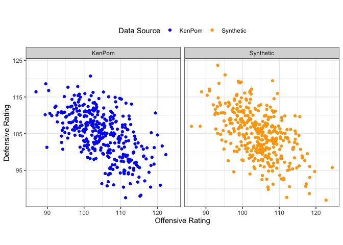
Verifying Actual and Synthetic Data Match
Plotting our synthetic data confirms that it convincingly resembles the KenPom 2023 data.
Generating and Simulating the Schedule
This section will be code-light and concept-heavy.
Generating Schedules
Random scheduling is quite easy to do. First, we randomly arrange the teams 1 to 362. Then, the teams are split in half and essentially “stacked” on top of each other, and each column corresponds to a game pairing. Finally, to create the next pairing of games the second row is shifted by one element to the right.
If that doesn’t make sense, here’s an example of how to generate a random schedule of two games for six teams.
First, we randomly sort the TeamIDs 1, 2, 3, 4, 5, 6, split in half, and then stack. This gives us our final schedule of three games for Week 1: 4 vs. 6, 2 vs. 3, and 5 vs. 1.
| Game 1 | Game 2 | Game 3 |
|---|---|---|
| 4 | 2 | 5 |
| 6 | 3 | 1 |
Now, we shift the bottom row to the right to obtain gameweek 2: 4 vs. 1, 2 vs. 6, and 5 vs. 3.
| Game 4 | Game 5 | Game 6 |
|---|---|---|
| 4 | 2 | 5 |
| 1 | 6 | 3 |
To schedule within conferences, we follow a similar method but allow the
helper function roundrobin from the Gmisc package to handle the
scheduling for us.8 We can now generate an arbitrary number of games
both in and out of conference for each team.
Simulating Games
This is where we have to make some assumptions (scary). Instead of the code, we can explain the game-simulation model in terms of the assumptions our game simulation model makes.
-
Each team’s expected points scored and allowed is a linear combination of their offensive efficiency and their opponent’s defensive efficiency, with equal weight given to each value.
-
To account for game-level variance (the best team doesn’t win 100 percent of the time!) we randomly sample from a Normal distribution with a mean equal to each team’s expected points from (1) and a standard deviation of 7.99 points. This value might seem extremely arbitrary, but it’s chosen for a very specific reason: when setting each team’s game-level standard deviation in points scored to 7.99, we end up with a mean absolute error on our season-long MOV predictions equal to 8.98 points — which just so happens to be the KenPom MAE for the 2023 season.
That’s it. Obviously, this is a pretty major simplification of basketball. In simulation-land, there is no home court advantage. Every team plays at the same tempo. Team ratings are constant throughout the season. Team rating uncertainty is also constant throughout the season. None of these assumptions in the simulations are true in real life. But they make it easier to draw conclusions about our toy efficiency-margin models.
Calculating Team Ratings
Essentially, for every game a team plays we look at their opponent’s season-long efficiencies excluding that game, compare that to the way the team played in the game, and find the difference. If Team 1 scored 1.20 PPP against Team 2 and Team 2 allowed 0.90 PPP on average in their other games, Team 1 receives a +0.30 offensive rating for that game. This is repeated for every game a team plays in a season, and then their offensive and defensive ratings are calculated by averaging their offensive and defensive performances in each game. Note that by virtue of the assumptions in game simulation, this very basic efficiency-margin system works — for example, because of the assumption that team ratings are stationary for the full season, we don’t need to worry about recency weighting.
Results
First, just to verify that the efficiency-rating system outlined in the previous section works in a perfect world, here’s a plot of what it looks like to simulate a very large number of games (150, in this case) against random teams and then use the team-ratings algorithm to estimate their performance. Remember, we’re looking for the estimated and actual ratings to match.
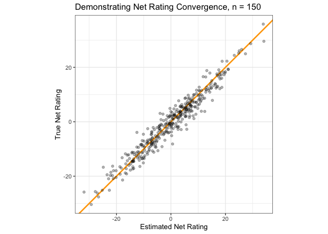
How does that chart look for our four scheduling options with approximately 30 games per team apiece? The random schedule does the best job producing net rating estimates which align with a team’s true rating. Assigning random conferences and then playing random games doesn’t seem to cause too much trouble, either. It’s when we start grouping conferences based on team strength that real problems begin to emerge; when we don’t have any non-conference cross-pollination to work with, our team rating estimates seem almost no better than random.
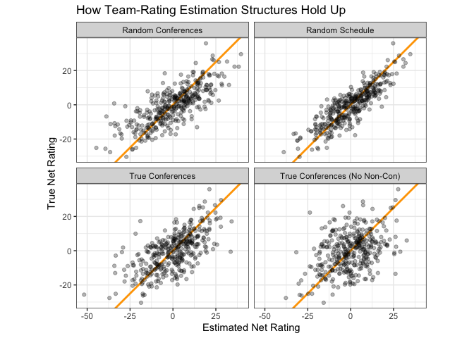
The below table puts some hard numbers to those charts — the mean absolute error of our estimates using the 30-game random schedule is only 5.30 rating points, but that number balloons to 8.18 when playing the approximate “actual” college basketball schedule of 10 non-con games and 20 conference games.
## # A tibble: 4 × 4
##   schedule_type                   mae  rmse pearson_r_sq
##   <chr>                         <dbl> <dbl>        <dbl>
## 1 Random Schedule                5.30  6.57        0.743
## 2 Random Conferences             7.47  9.65        0.586
## 3 True Conferences               8.18 10.4         0.415
## 4 True Conferences (No Non-Con)  9.88 12.6         0.158
What’s the source of this error? It’s the “bubble” effect: when teams play insular groupings of teams on their schedule, it becomes much more challenging to draw conclusions about how they relate to the larger whole. If — for example — ACC teams only played other ACC teams, it would be impossible to figure out how the ACC compares to the rest of college basketball writ large.
Inter-conference play is the glue that holds any predictive rating system together.
The below chart looks at how well the efficiency rating system identifies the true conference strengths within the data. Based on what we know about the “bubble” effect, we should expect the system to do pretty well at identifying true conference strength with the fully random schedule and the randomized-conferences schedule, though the latter will have more variance as its results are essentially based on fewer games. For the schedule with 10 non-con games and then 20 games against “true” conferences, the conference strength estimates should be biased towards zero because once teams enter conference play there’s no opportunity for the conference to gain or lose strength. And for the schedule with 30 conference games, we don’t expect any conference strength estimates to deviate from zero because there are no non-conference games to base those estimates on.
The data pretty much confirm these priors:
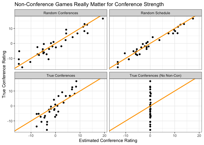
How do we get around the bubble problem? Remember, the raw actual ratings for college basketball correspond to the “True Conferences” panel in the above plot. Option 1 is adding some prior estimates of conference strength based on previous seasons to our estimates of each team’s strength in a conference. This gets us closer to the ground truth than the unadjusted option — and I suspect is the way most public predictive rating systems work — but there is something frustrating about teams potentially being penalized or rewarded by the selection committee based on the performance of other teams from other seasons.9 Option 2 is a revision of the way college basketball scheduling works to incorporate more non-conference games into the season.
Conclusions
What can we learn from this experiment?
The exact numbers on team ratings should be taken with a grain of salt. Even if a rating system’s estimates of team strength were perfectly accurate, the variance inherent to a short 30-game season (and additional variance incurred by limiting two-thirds of that schedule to games between conference “bubbles”) means that offensive and defensive efficiency estimates will always have quite a bit of unavoidable error. This issue is only exacerbated by the frequent usage of ordinal ranks when describing team ratings via a specific rating system (i.e. incessant “Only teams in the top X on KenPom can win the NCAA Tournament!” tweets), a practice which is narratively very satisfying but not particularly meaningful in practice.
The numbers in this study can be used as a grain-of-salt upper bound on predictive-metric error. Every team-rating system out there is smarter than this naive efficiency rating system.10 But that 8.11 MAE value is a useful benchmark to keep in mind — if you think that (your predictive rating system du jour) is twice as good as this system, that’s still a mean absolute error of at least four points of net rating. Predictive rating systems are better than just about anything else at identifying how good teams are, but they aren’t perfect, or really anywhere near perfect — something that all of their creators would tell you in a heartbeat.
As for the conference question? It’s an unavoidable part of the structure of college basketball that conference play will exist and that there will be a hierarchy between conferences. This damages predictive team rating systems in two ways compared to a totally randomized schedule. First, it increases the variance of our team strength estimates in general. Second, it limits the information we can glean about relative conference strength. This necessitates the hacky solution of using conference strength in previous seasons to inform estimates of conference strength in a given season — the alternative is conference-strength estimates incredibly sensitive to non-con play — which can be very frustrating from a team’s perspective: why are we being penalized for what a team last season did or didn’t do?
The particulars of the college basketball schedule — specifically, the fact that almost all pre-tournament non-conference games are played early in the season — also eliminate the potential for team rating systems to pick up on differences in how different teams improve over the course of the season by conference. That’s another concern Boeheim et. al. have raised on more than one occasion.
Where do we go from here?
What’s the best fix? I’m partial to a solution I read about on Ken Pomeroy’s blog a few years ago but am unable to track down at the moment: hold some slots open later in the season for teams to schedule a few non-conference games around the end of the season.11 This lets bubble teams from mid-majors potentially pick up big resume wins. It further informs predictive rating systems through the inclusion of more non-conference games, which we’ve established are the lifeblood of team rating estimation. And it even allows for the potential detection of an interaction between conference and team improvement over the course of the season. Best of all, it’s not a drastic enough shakeup to actually cause major issues in the college basketball landscape, so it feels feasible.
Leaving a week empty in the middle of conference season to allow teams to schedule their own non-con games is the best bang-for-buck solution to the insular conference problem. It would make team rating systems more accurate, less reliant on previous-season data, and generally more effective tools for selecting NCAA Tournament games. It would add a ton of entertaining games to the schedule as strong mid-majors and middle-of-the-road P6 teams have mutual interest in scheduling matchups with one another. There have been plenty of major changes to the college basketball landscape over the previous few seasons. What’s one more?
Full code available in this repository: https://github.com/bbwieland/cbb-team-rating-system-analysis
-
https://x.com/WRALBobHolliday/status/1753996220937216348?s=20 ↩
-
https://www.si.com/college/pittsburgh/basketball/pitt-panrhers-jeff-capel-calls-out-acc-disrespect ↩
-
Full rankings available here: https://barttorvik.com/cgi-bin/ncaat.cgi?conlimit=&yrlow=2010&yrhigh=2023&type=conf&sort=1 ↩
-
https://www.kaggle.com/competitions/mens-march-mania-2022/discussion/317316 ↩
-
The reason the games don’t exactly add up to 30 for each team is because of conferences with odd numbers of teams, which necessarily require “bye weeks.” Some teams will play 31-32 games, some will play 28-29, but in the aggregate the total number of games played will be almost identical to Experiment 1. ↩
-
The two independent teams, Chicago State and Hartford, were assigned to the NEC to make sure there wasn’t actually a two-team-conference. This has a negligible effect on the results of the study. ↩
-
I’ve kept this file purposefully code-light and focused on the results above all else. The full code will be included in a separate GitHub repository which will be linked at the bottom of the article. ↩
-
This is because I am bad at writing efficient code. ↩
-
When I built a game projection system for men’s college basketball last season, this was the approach I employed: reweighting the rankings to add approximately 40% of a conference’s average rating in the previous season to all of its ratings for the current season. Warts and all, it does make forecasts more accurate. ↩
-
Except the AP Poll, ba dum tss. ↩
-
If anyone finds this article, please send it to me. ↩