Reel Analytics is a sports tech company with at least 18,000 Twitter followers, internationally renowned sports scientists on staff, and glowing testimonials from multiple college coaches: Deion Sanders described their metrics as “foundational” to his talent evaluation process. Using computer vision, Reel extracts tracking metrics from broadcast video and uses these metrics for player evaluation data which are supplied to its clients: NFL scouts, agents, and major college football programs.
With so much tracking data traditionally paywalled behind vendors or excluded from the public view entirely1, it’s a privilege to get a glance at what’s going on under the hood with these high-level computer vision tracking data models. Reel already generously provide an overview of their process in a 31-page whitepaper.2 Recently, they went a step further: posting 40-yard dash forecasts for over 100 NFL Draft prospects on their Twitter account.
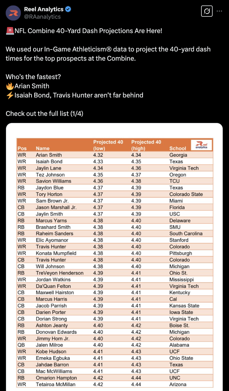
I’ve always been curious how the accuracy of these computer vision models holds up when put to the test, and public predictions mean public validation! I scraped the four tweets put out by Reel Analytics containing their predicted 40-yard dash times and combined them with observed data from the NFL API.3
Model Calibration
The figures reported by Reel Analytics on Twitter provided extremely narrow confidence intervals. For some players, the variation between the “low” and “high” projected 40-yard dash times spanned 0.03 seconds, while for others like Texas QB Quinn Ewers the model predicted an incredibly narrow confidence interval of 0.01 seconds.
After clicking on that tweet containing Ewers’s projected 40-yard dash range – 4.48 to 4.49 seconds – Grok AI prompted me with a potential question: “Are projections historically accurate?” Rather than ask Grok for the answer and generate some AI slop response while burning some trees down in the Amazon to power Grok’s GPUs while I’m at it, I just checked the actual calibration rates of the model against observed 2025 40-yard dash times.
This is pretty simple to do! Given the lower & upper bounds for each projection provided by Reel Analytics’s tweets, we can simply see if the actual 40 time each player ran falls within the provided confidence interval. Note that Reel doesn’t claim any particular level of confidence on these ranges, simply providing a “low” and “high” projection. It’s statistical convention4 to present 95% confidence intervals, so my initial assumption was that these were 95% CIs, but that feels like an unreasonably high standard. If I actually timed all of these 40-yard dashes with a stopwatch, I don’t think I’d get within 0.02 seconds of the correct time 95% of the time!
Regardless, the data speak for themselves. Of the 96 pairs of Reel Analytics predictions and observed 40-yard dash times, just 10 fell within the supplied confidence intervals, good for a 10.4% calibration rate.
Code for the plot
``` r total_preds = nrow(preds) correct_preds = sum(preds$value_within_ci) plot_title = "Reel Analytics 40-Yard Dash Model Calibration" plot_subtitle = paste0(correct_preds, " of " ,total_preds, " 40-yard dash times fell within the confidence interval.") ggplot(preds, aes(y=fct_reorder(paste0(player, " (", position, ")"), desc(pred_lower)))) + geom_point(aes(x = pred_lower)) + geom_point(aes(x = pred_upper)) + geom_segment(aes(x = pred_lower, xend = pred_upper)) + geom_point(aes(x = obs_time), color = "red") + theme_bw() + labs(x = "40-Yard Dash Time", y = NULL, title = plot_title, subtitle = plot_subtitle) + theme(plot.title = element_text(face = "bold")) ```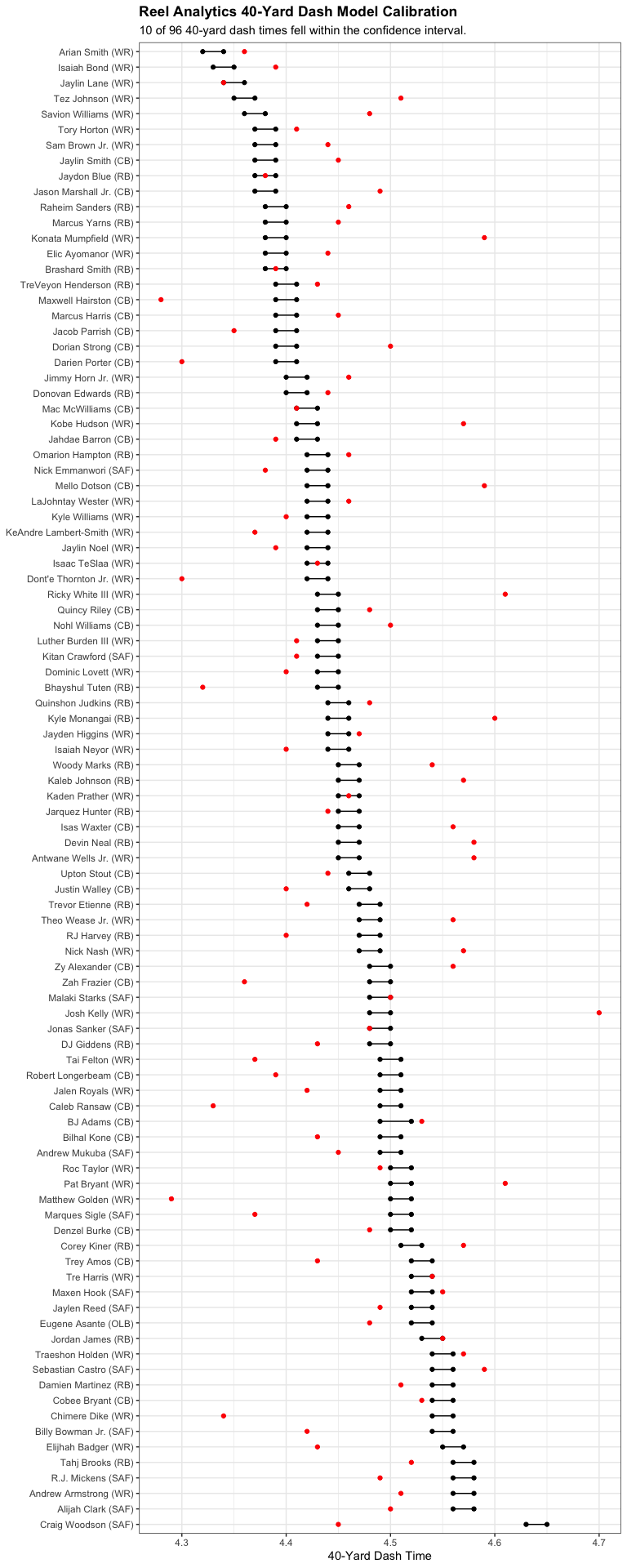
There’s not really a generous interpretation of these numbers: only about 1 in 10 predictions fell within the reported confidence interval! Clearly, the reported intervals are far too precise.
We can calculate what these confidence intervals “should have” been, essentially answering the question “How wide do our confidence intervals on our predictions need to be for them to contain X% of the observed values?” Again, this is pretty easy to do! We simply:
-
Take the predicted point estimate of each player’s 40 time as the average of their lower & upper bound forecasts from the Reel Analytics tweets.
-
Find the smallest possible confidence interval width which contains some percentage of the observed data, given our predictions.5
Code for finding minimum viable confidence intervals
``` r get_observed_calibration <- function(interval_width) { interval_preds <- preds %>% mutate(interval_lower = pred_value - interval_width / 2, interval_upper = pred_value + interval_width / 2) %>% mutate(value_within_interval = ifelse(obs_time <= interval_upper & obs_time >= interval_lower, 1, 0)) return(mean(interval_preds$value_within_interval)) } ``` ``` r find_necessary_ci_width <- function(desired_calibration, step_size = 0.005) { calibration_pct = 0 interval = 0.01 while (calibration_pct <= desired_calibration) { calibration_pct <- get_observed_calibration(interval_width = interval) if (calibration_pct < desired_calibration) { interval = interval + step_size } } return(interval) } ``` ``` r potential_calibration_rates <- c(0.5, 0.8, 0.9, 0.95) necessary_intervals <- c() for (rate in potential_calibration_rates) { necessary_intervals <- c(necessary_intervals, find_necessary_ci_width(rate)) } calibration_df <- data.frame(calibration_rate = potential_calibration_rates, interval_width = necessary_intervals) ``` ``` r calibration_df %>% gt::gt() %>% gt::cols_label(calibration_rate ~ 'Calibration Rate', interval_width ~ "Confidence Interval") %>% gt::fmt_percent(calibration_rate, decimals = 0) %>% gt::cols_align('center') ```I found these necessary confidence interval widths for a few possible calibration rates. As it turns out, 50 percent of the observed 40-yard dash times fell within +/- 0.06 seconds of the Reel Analytics prediction – a far cry from the supplied confidence intervals of +/- 0.01 seconds, but not bad! To achieve that 95 percent confidence level common in both statistical literature and the popular imagination, we need a confidence interval of +/- 0.19 seconds.
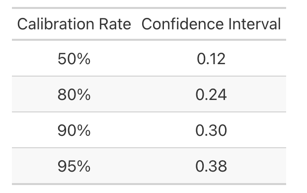
For Quinn Ewers, this would’ve given us a prediction interval with a lower bound of 4.30 and an upper bound of 4.68. For context, Devon Achane ran a 4.32 and Matt Araiza ran a 4.68 – I guess “we are 95 percent confident Quinn Ewers’s 40-yard dash will be slower than an explosive dual-threat receiving back, but faster than Kansas City’s punter” probably wouldn’t generate quite as much engagement. Regardless, the prediction would’ve been wrong: Ewers opted out of the 40.
Model Performance
Even if the model’s predictions are too hyper-specific, that doesn’t necessarily mean they’re bad! After all, Reel uses objective evaluative metrics extracted by AI-powered tracking technology along with objective advanced performance metrics according to their website, and those must be hard to beat. There’s a chance the underlying model holds up and it’s just being presented with too much confidence online – and if being overconfident online is a crime, most social media users are probably going to prison.
In fact, Reel’s CEO reported big wins for the model. According to his LinkedIn post, “most athletes performed close to their projected 40-yard dash times, but a few outliers ran faster or slower than expected, possibly due to field conditions, reaction time, and/or combine-specific training factors.”
What’s tricky here, though, is determining what “close” means. I don’t have any context for the reported value that 85% of Reel’s DB projections fell within 0.10 seconds of the observed 40 time. Is that good? What is good for 40-yard dash projections, anyways?
To get an answer here, I decided it was time to pull in some objective advanced performance metrics of my own and create another 40-yard dash forecasting model. Armed with 2024 NFL Combine data downloaded from Football Reference6 as my training set, I set up two formidable competitor models.
-
Position Baseline: This model predicts the average 40-yard dash time for each position group in 2024. In R syntax, it’s just
lm(dash ~ position) -
Weight Baseline: Wait, don’t skinnier guys run faster? To model this, I standardized each player’s weight by position group – if a wide receiver weighed 180 pounds and the average WR in the 2024 Combine data weighed 195 pounds, his “adjusted weight” would be -15 pounds. Then, I fit a univariate linear regression mapping this adjusted weight to 40-yard dash time. In R syntax,
lm(dash ~ adjusted_weight).
(Apologies for breaking kayfabe momentarily, but these models are terrible. Just embarrassingly bad. I mean, if you can’t do better than just looking at a guy’s listed position or his listed weight to project his 40-yard dash time, what are you doing? I bet any scout – or probably any sufficiently committed college football fan – could beat these numbers easily.)
Fitting and validating the baseline models
``` r clean_train <- train %>% janitor::clean_names() %>% # Only model the positions included in '25 combine data. dplyr::filter(pos %in% preds$position) %>% dplyr::select(player, position = pos, weight = wt, dash = x40yd) %>% # Exclude players without 40-yard dash times. dplyr::filter(!is.na(dash)) # Calculate positional average 40-yard dash times in 2024. weight_avgs <- clean_train %>% dplyr::group_by(position) %>% dplyr::summarise(avg_weight = mean(weight)) # Add weights relative to position group in 2024. prep_train <- clean_train %>% dplyr::inner_join(weight_avgs, by = 'position') %>% dplyr::mutate(weight = weight - avg_weight) # Fit two baseline models: # - one that just predicts the average 40 time for each position group. # - a single-variable linear regression on position-standardized weight. position_baseline <- lm(dash ~ position, data=prep_train) weight_baseline <- lm(dash ~ weight, data=prep_train) ``` I took these models for a spin against the full technical might of Reel Analytics’s computer-vision-based tracking data, expecting a rout for the machines.[^7] Armed with predictions from each of my two models as well as Reel’s forecasts, I compared the performance of each set of 2025 Combine predictions using the three accuracy metrics supplied in the Reel CEO’s LinkedIn post above, as well as two more traditional machine learning metrics: mean absolute error and root mean squared error.[^8] ``` r clean_preds <- preds %>% # Only including positions we can predict over (i.e. that ran a 40 in '24) dplyr::filter(position %in% clean_train$position) %>% # We use the '24 positional average 40 times, to prevent data leakage. inner_join(weight_avgs, by = 'position') %>% mutate(weight = weight - avg_weight) full_pred_df <- clean_preds %>% # Add predictions for each of the baseline models. dplyr::mutate(baseline_pred = predict(position_baseline, clean_preds), weight_pred = predict(weight_baseline, clean_preds)) %>% # Add model residuals. dplyr::mutate(reel_model_residual = obs_time - pred_value, position_baseline_residual = obs_time - baseline_pred, weight_baseline_residual = obs_time - weight_pred) ``` ``` r preds_long <- full_pred_df %>% dplyr::select(player, position, college, reel_model_residual, position_baseline_residual, weight_baseline_residual) %>% tidyr::pivot_longer(cols = c(reel_model_residual, position_baseline_residual, weight_baseline_residual), names_to = 'model_type', values_to = 'residual', names_transform = function (x) gsub("_residual", '', x)) ``` ``` r pred_performance_table <- preds_long %>% group_by(model_type) %>% summarise(hi_accuracy = sum(abs(residual) <= 0.05) / n(), md_accuracy = sum(abs(residual) <= 0.10 & abs(residual) >= 0.05) / n(), lo_accuracy = sum(abs(residual) > 0.10) / n(), mae = mean(abs(residual)), rmse = sqrt(mean(residual ^ 2))) %>% mutate(model_type = gsub("_", " ", model_type)) %>% mutate(model_type = stringr::str_to_title(model_type)) ``` ``` r pred_performance_table %>% gt::gt() %>% gt::cols_label(hi_accuracy ~ "<= 0.05", md_accuracy ~ "0.05-0.10", lo_accuracy ~ "> 0.10", model_type ~ 'Model', mae ~ "MAE", rmse ~ "RMSE") %>% gt::tab_spanner('Accuracy', columns = gtExtras::contains('accuracy')) %>% gt::fmt_percent(gtExtras::contains('accuracy'), decimals = 0) %>% gt::cols_align('center') %>% gt::fmt_number(c(mae, rmse), decimals = 4) ```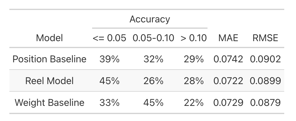
Wow! Sure, by LinkedIn standards we got our asses kicked in “High Accuracy” predictions: 45% of Reel’s predictions fell within 0.05 seconds of the observed 40-yard dash time, while just 39% of predictions from our position-group model and 33% of predictions from our player-weight model achieved that level of accuracy. However, Reel missed by at least 0.10 seconds 28% of the time, while our weight baseline model only made errors that large 22% of the time. By mean absolute error, Reel only beat our baseline weight model by 0.0007 points. And by root mean squared error – the metric most machine learning models optimize against7, and one that punishes big misses harshly – our weight baseline model actually beats the Reel Analytics model with all its bells and whistles.
Takeaways
If you’re a college football team, Reel Analytics offers on-demand analytics for an unlimited number of college players under their “Unlimited” plan. A yearly subscription to this plan costs $14,999. In light of the performance of Reel’s 40-yard dash model, the following courses of action may make sense:
-
Stop printing the weights of your players in your gameday programs, and instead charge $14,999 for those numbers. After all, they’re about as predictive as the proprietary 40-yard dash model seems to be.
-
Since predicting 40-yard dash times based on only a player’s position group performs slightly worse than Reel’s model, maybe price that information around $10,000.
-
Cancel your Reel Analytics subscription and spend the money on paying stipends to the dozens of college students at your university who are dying to break into the sports analytics field and would happily work for free on these exact problems.
If you’re a college player, you can either purchase a $25 Fastest Player Challenge max-speed analysis or a Comprehensive Athletic Evaluation for $199. If the school recruiting you doesn’t want to see these data, don’t pay for them. If the school recruiting you does want to see these data, commit to a different school.
If you’re a sports tech investor looking to invest, don’t.
Note: A previous version of this table contained incorrect values in the “Medium” accuracy range of the model evaluation table. This error has now been fixed, and the table values displayed are correct.
-
Source: I work in baseball. ↩
-
Some edits for conciseness may have benefited this whitepaper – for example, I don’t think we needed to spend two-thirds of page 22 defining velocity – but I digress. ↩
-
It’s beyond the scope of this piece to describe how I did this, but essentially I ripped an old Thomas Mock blog post to perform OCR on the Reel Analytics twitter images & then post-processed some of the obviously wrong values to clean everything up. There’s a good chance some data get dropped due to OCR errors, but it doesn’t affect many values & doesn’t systemically affect the results. ↩
-
Although this is kinda bullshit – see https://github.com/easystats/bayestestR/discussions/250 ↩
-
I am bad at programming and also lazy, so I did this with non-vectorized
forloops, but you can definitely do this more efficiently. Also, my sincerest apologies that the code embeds do not work and are essentially unreadable. ↩ -
Sports Reference sites do not allow scraping, so to get the data I first downloaded it as an Excel workbook, opened it in read-only mode using my personal copy of Microsoft Excel which now no longer allows me to save files without a Microsoft Office subscription, copy pasted it into Google Sheets, and saved that file as a csv. Real professional stuff, I know. ↩
-
Don’t put too much stock into this, though, since it’s mostly a function of most gradient descent optimizers working better when evaluated against L2 loss. There’s no epistemic reason RMSE is the Holy Grail, just computational reasons. ↩